CoCalc Logo Icon
DocsShareSupport News Sign UpSign In
Views: 100
Image: ubuntu2004
Embed | Download | Raw |
Kernel: Python 3 (ipykernel)
import random import math from IPython.core.display import SVG import pyomo.environ as pyo from pysat.solvers import Solver from pysat.formula import CNF import py_svg_combinatorics as psc from ipywidgets import widgets, HBox from collections import Counter from pprint import pprint from random import randint import numpy as np from IPython.display import IFrame import IPython from copy import copy import os from pathlib import Path np.set_printoptions(precision=2) np.set_printoptions(suppress=True) nbname = '' try: nbname = __vsc_ipynb_file__ except: if 'COCALC_JUPYTER_FILENAME' in os.environ: nbname = os.environ['COCALC_JUPYTER_FILENAME'] title_ = Path(nbname).stem.replace('-', '_').title() IFrame(f'https://discopal.ispras.ru/index.php?title=Hardprob/{title_}&useskin=cleanmonobook', width=1280, height=300)
def print_solution(m): for v in m.component_data_objects(pyo.Var): if v.value and v.value > 0: print(str(v), v.value)
m = n = np.random.randint(2, 3) def generate_random_data_for_maxqp(n): m = n # Линейные ограничения для допустимой области A = np.random.rand(m, n) b = 10*np.ones(m) #np.floor(1/np.random.rand(m)) M = np.random.rand(m, n) Q = np.dot(M, M.T) # симметричная положительно-полуопределенная c = np.random.rand(n) return A, Q, c, b A, Q, c, b = generate_random_data_for_maxqp(n) A, Q, c, b
(array([[0.81, 0.01], [0.13, 0.38]]), array([[0.04, 0.15], [0.15, 0.69]]), array([0.38, 0.57]), array([10., 10.]))

11

def get_model_bbl(A, b, Q, c): m = pyo.ConcreteModel() m.m, m.n = A.shape # на всякий случай, возьмем с собой m.A = A m.Q = Q m.b = b m.c = c m.I = range(m.m) # m.J = range(m.n) upper_bound_x = math.ceil(max([b[i] / min([m.A[i, j] for j in m.I]) for i in m.I])) m.u = upper_bound_x #16 #256 bin_len = math.ceil(math.log(m.u)/math.log(2)) m.K = range(bin_len) m.x = pyo.Var(m.I, domain=pyo.NonNegativeIntegers) @m.Constraint(m.I) def не_больше(m, i): return sum(A[i, j] * m.x[j] for j in m.I) <= b[i] m.t_ik = pyo.Var(m.I, m.K, domain=pyo.Binary) @m.Constraint(m.I) def t_будет_бинарным_разложением_x(m, i): return m.x[i] == sum(2**k * m.t_ik[i, k] for k in m.K) # Бинарное произведение y_ikjl = t_ik * t_jl m.y_ikjl = pyo.Var(m.I, m.K, m.I, m.K, domain=pyo.Binary) @m.Constraint(m.I, m.K, m.I, m.K, [7, 8, 9, 10, 11, 13]) def y_ikjl_constraint_A(m, i, k, j, l, c): if c == 7 and m.Q[i,j] < 0: return m.y_ikjl[i, k, j, l] <= m.t_ik[i, k] if c == 8 and m.Q[i,j] < 0: return m.y_ikjl[i, k, j, l] <= m.t_ik[j, l] if c == 9 and m.Q[i,j] > 0: return m.y_ikjl[i, k, j, l] >= m.t_ik[i, k] + m.t_ik[j, l] - 1 if c == 10 and m.Q[i,j] > 0: return m.y_ikjl[i, k, j, l] >= 0 if c == 11 and m.Q[i,j] != 0 and i < j: return m.y_ikjl[i, k, j, l] == m.y_ikjl[j, l, i, k] if c == 13 and m.Q[i,i] != 0 and k < l: return m.y_ikjl[i, k, i, l] == m.y_ikjl[i, l, i, k] return pyo.Constraint.Skip @m.Constraint(m.I, m.K, [12]) def y_ikjl_constraint_B(m, i, k, c): if c == 12 and m.Q[i,i] != 0: return m.y_ikjl[i, k, i, k] == m.t_ik[i, k] return pyo.Constraint.Skip @m.Objective(sense=pyo.maximize) def сложная_побитовая_сумма(m): return sum( Q[i, j] * sum(2**(k+l) * m.y_ikjl[i, k, j, l] for k in m.K for l in m.K ) for i in m.I for j in m.I) return m m = get_model_bbl(A, b, Q, c) m.u #m.pprint()
1056
solver = pyo.SolverFactory('cbc') solver.solve(m).write()
# ========================================================== # = Solver Results = # ========================================================== # ---------------------------------------------------------- # Problem Information # ---------------------------------------------------------- Problem: - Name: unknown Lower bound: 3302336.2440436 Upper bound: 3302336.2440436 Number of objectives: 1 Number of constraints: 162 Number of variables: 182 Number of binary variables: 506 Number of integer variables: 508 Number of nonzeros: 182 Sense: maximize # ---------------------------------------------------------- # Solver Information # ---------------------------------------------------------- Solver: - Status: ok User time: -1.0 System time: 0.15 Wallclock time: 0.09 Termination condition: optimal Termination message: Model was solved to optimality (subject to tolerances), and an optimal solution is available. Statistics: Branch and bound: Number of bounded subproblems: 0 Number of created subproblems: 0 Black box: Number of iterations: 1 Error rc: 0 Time: 0.7625322341918945 # ---------------------------------------------------------- # Solution Information # ---------------------------------------------------------- Solution: - number of solutions: 0 number of solutions displayed: 0
#print_solution(m) print(m.x.extract_values())
{0: 0.0, 1: 26.0}
[m.x[i].value for i in m.I]
[0.0, 26.0]

Упражнения

  • Найти кое-что пропущеное в постановке
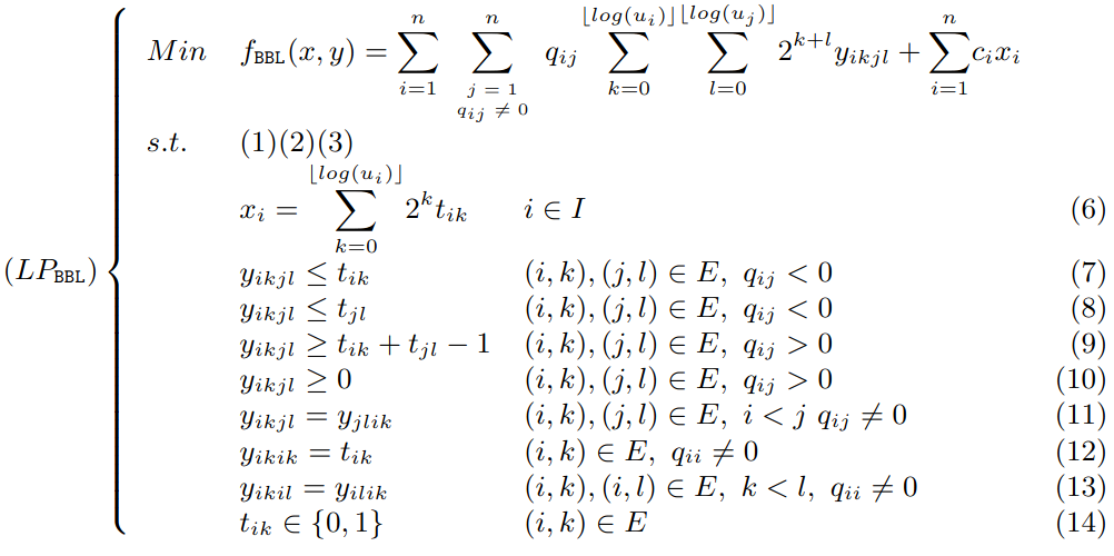
 get_model_bbl (мелочь, так, на внимательность)

Разобраться в ограничениях BBL

  • Написать комментарии зачем они.

  • Можно уменьшить их число?

Сделать отдельно линеаризацию BIL

т.е. написать функцию get_model_bil «binary integer linerization» из статьи

А что с библиотеками для решения квадратичного программирования?

import picos as pic import matplotlib.pyplot as plt import scipy import cvxopt as cvx import cvxpy as cp

Простой пример с CVXPY

Не Pyomo, но схожий язык.

Оптимизационные переменные

x = cp.Variable() y = cp.Variable()

Ограничения

constraints = [x + y == 1, x - y >= 1]

Целевая функция

obj = cp.Minimize((x - y)**2)

Решаем

prob = cp.Problem(obj, constraints) prob.solve() prob.status, prob.value, x.value, y.value
('optimal', 1.0, array(1.), array(0.))
Q = np.array([[0, 1], [1, 0]]) Q
array([[0, 1], [1, 0]])
y = cp.Variable(2, integer=True) obj = cp.quad_form(y, Q) constraits = [y >= -2, y <= 2] prob = cp.Problem(cp.Maximize(obj), constraits) # prob = cp.Problem(cp.Minimize(obj), constraits) print(prob) prob.solve() #solver=cp.SCIP
maximize QuadForm(var45, [[0.00 1.00] [1.00 0.00]]) subject to -2.0 <= var45 var45 <= 2.0
--------------------------------------------------------------------------- DCPError Traceback (most recent call last) /var/data/cocalc/1d588dae-0d14-422a-88b4-c470ec2c8303/hard-problems-formulations/maximum-quadratic-programming.ipynb Cell 24 line 8 <a href='vscode-notebook-cell://xn--17-6kce2c.xn--80apqgfe.xn--p1ai/var/data/cocalc/1d588dae-0d14-422a-88b4-c470ec2c8303/hard-problems-formulations/maximum-quadratic-programming.ipynb#X32sdnNjb2RlLXJlbW90ZQ%3D%3D?line=5'>6</a> # prob = cp.Problem(cp.Minimize(obj), constraits) <a href='vscode-notebook-cell://xn--17-6kce2c.xn--80apqgfe.xn--p1ai/var/data/cocalc/1d588dae-0d14-422a-88b4-c470ec2c8303/hard-problems-formulations/maximum-quadratic-programming.ipynb#X32sdnNjb2RlLXJlbW90ZQ%3D%3D?line=6'>7</a> print(prob) ----> <a href='vscode-notebook-cell://xn--17-6kce2c.xn--80apqgfe.xn--p1ai/var/data/cocalc/1d588dae-0d14-422a-88b4-c470ec2c8303/hard-problems-formulations/maximum-quadratic-programming.ipynb#X32sdnNjb2RlLXJlbW90ZQ%3D%3D?line=7'>8</a> prob.solve() #solver=cp.SCIP File ~/hard-problems-formulations/.venv/lib64/python3.11/site-packages/cvxpy/problems/problem.py:503, in Problem.solve(self, *args, **kwargs) 501 else: 502 solve_func = Problem._solve --> 503 return solve_func(self, *args, **kwargs) File ~/hard-problems-formulations/.venv/lib64/python3.11/site-packages/cvxpy/problems/problem.py:1072, in Problem._solve(self, solver, warm_start, verbose, gp, qcp, requires_grad, enforce_dpp, ignore_dpp, canon_backend, **kwargs) 1069 self.unpack(chain.retrieve(soln)) 1070 return self.value -> 1072 data, solving_chain, inverse_data = self.get_problem_data( 1073 solver, gp, enforce_dpp, ignore_dpp, verbose, canon_backend, kwargs 1074 ) 1076 if verbose: 1077 print(_NUM_SOLVER_STR) File ~/hard-problems-formulations/.venv/lib64/python3.11/site-packages/cvxpy/problems/problem.py:646, in Problem.get_problem_data(self, solver, gp, enforce_dpp, ignore_dpp, verbose, canon_backend, solver_opts) 644 if key != self._cache.key: 645 self._cache.invalidate() --> 646 solving_chain = self._construct_chain( 647 solver=solver, gp=gp, 648 enforce_dpp=enforce_dpp, 649 ignore_dpp=ignore_dpp, 650 canon_backend=canon_backend, 651 solver_opts=solver_opts) 652 self._cache.key = key 653 self._cache.solving_chain = solving_chain File ~/hard-problems-formulations/.venv/lib64/python3.11/site-packages/cvxpy/problems/problem.py:898, in Problem._construct_chain(self, solver, gp, enforce_dpp, ignore_dpp, canon_backend, solver_opts) 896 candidate_solvers = self._find_candidate_solvers(solver=solver, gp=gp) 897 self._sort_candidate_solvers(candidate_solvers) --> 898 return construct_solving_chain(self, candidate_solvers, gp=gp, 899 enforce_dpp=enforce_dpp, 900 ignore_dpp=ignore_dpp, 901 canon_backend=canon_backend, 902 solver_opts=solver_opts, 903 specified_solver=solver) File ~/hard-problems-formulations/.venv/lib64/python3.11/site-packages/cvxpy/reductions/solvers/solving_chain.py:217, in construct_solving_chain(problem, candidates, gp, enforce_dpp, ignore_dpp, canon_backend, solver_opts, specified_solver) 215 if len(problem.variables()) == 0: 216 return SolvingChain(reductions=[ConstantSolver()]) --> 217 reductions = _reductions_for_problem_class(problem, candidates, gp, solver_opts) 219 # Process DPP status of the problem. 220 dpp_context = 'dcp' if not gp else 'dgp' File ~/hard-problems-formulations/.venv/lib64/python3.11/site-packages/cvxpy/reductions/solvers/solving_chain.py:132, in _reductions_for_problem_class(problem, candidates, gp, solver_opts) 129 elif problem.is_dqcp(): 130 append += ("\nHowever, the problem does follow DQCP rules. " 131 "Consider calling solve() with `qcp=True`.") --> 132 raise DCPError( 133 "Problem does not follow DCP rules. Specifically:\n" + append) 134 elif gp and not problem.is_dgp(): 135 append = build_non_disciplined_error_msg(problem, 'DGP') DCPError: Problem does not follow DCP rules. Specifically: The objective is not DCP. Its following subexpressions are not: QuadForm(var45, [[0.00 1.00] [1.00 0.00]])

Визуализируем эту матрицу

n_points = 5 u = np.linspace(-2, 2, n_points) u
array([-2., -1., 0., 1., 2.])
x1, x2 = np.meshgrid(u, u) x1, x2
(array([[-2., -1., 0., 1., 2.], [-2., -1., 0., 1., 2.], [-2., -1., 0., 1., 2.], [-2., -1., 0., 1., 2.], [-2., -1., 0., 1., 2.]]), array([[-2., -2., -2., -2., -2.], [-1., -1., -1., -1., -1.], [ 0., 0., 0., 0., 0.], [ 1., 1., 1., 1., 1.], [ 2., 2., 2., 2., 2.]]))
all_x = list(np.array([x1,x2]) for x1, x2 in zip(np.ravel(x1), np.ravel(x2))) all_x
[array([-2., -2.]), array([-1., -2.]), array([ 0., -2.]), array([ 1., -2.]), array([ 2., -2.]), array([-2., -1.]), array([-1., -1.]), array([ 0., -1.]), array([ 1., -1.]), array([ 2., -1.]), array([-2., 0.]), array([-1., 0.]), array([0., 0.]), array([1., 0.]), array([2., 0.]), array([-2., 1.]), array([-1., 1.]), array([0., 1.]), array([1., 1.]), array([2., 1.]), array([-2., 2.]), array([-1., 2.]), array([0., 2.]), array([1., 2.]), array([2., 2.])]
Z = np.array([ np.dot(x.T, np.dot(Q, x)) for x in all_x]) Z = Z.reshape(x1.shape) Z
array([[ 8., 4., 0., -4., -8.], [ 4., 2., 0., -2., -4.], [ 0., 0., 0., 0., 0.], [-4., -2., 0., 2., 4.], [-8., -4., 0., 4., 8.]])
fig = plt.figure(figsize=(6,6)) ax = fig.add_subplot(111, projection='3d') plt.figure() ax.plot_surface(x1, x2, Z)
<mpl_toolkits.mplot3d.art3d.Poly3DCollection at 0x7f0a9b53dd20>
Image in a Jupyter notebook
<Figure size 432x288 with 0 Axes>

Увы, библиотеки работают с выпуклыми-коническими функциями и ограничениями.

A, _, c, b = generate_random_data_for_maxqp(2) A, Q, c, b
(array([[0.24, 0.5 ], [0.06, 0.13]]), array([[0, 1], [1, 0]]), array([0.57, 0.17]), array([10., 10.]))
m = get_model_bbl(A, b, Q, c) solver.solve(m).write()
# ========================================================== # = Solver Results = # ========================================================== # ---------------------------------------------------------- # Problem Information # ---------------------------------------------------------- Problem: - Name: unknown Lower bound: 130050.0 Upper bound: 130050.0 Number of objectives: 1 Number of constraints: 0 Number of variables: 0 Number of binary variables: 144 Number of integer variables: 146 Number of nonzeros: 0 Sense: maximize # ---------------------------------------------------------- # Solver Information # ---------------------------------------------------------- Solver: - Status: ok User time: -1.0 System time: 0.01 Wallclock time: 0.02 Termination condition: optimal Termination message: Model was solved to optimality (subject to tolerances), and an optimal solution is available. Statistics: Branch and bound: Number of bounded subproblems: 0 Number of created subproblems: 0 Black box: Number of iterations: 0 Error rc: 0 Time: 0.12091326713562012 # ---------------------------------------------------------- # Solution Information # ---------------------------------------------------------- Solution: - number of solutions: 0 number of solutions displayed: 0
[m.x[j].value for j in m.x]
[0.0, 0.0]

Упражнения

  • Сделать генерацию данных подходящих для решения библиотеками cvxpy, cvxopt, picos (коническое-выпуклое) и прорешать и этими библиотеками, и через линеаризацию, сравнить, возможно найти ошибки. (достаточно добавить еще одну библиотеку, не обязательно перебирать все, или даже для имеющихся cvxpy это проделать)

  • Кстати, pyomo тоже умеет в квадратичное программирование, см. например 1, но не факт что со всеми солверами — тоже надо потестировать.